In previous posts we have discussed about the causes of the non-backdrivability in robotic actuators, the efficiency of most common reducers and the conditions under which a ballscrew becomes backdrivable. Here we will take a closer look into the effects of the non-backdrivability into the force control.
We can distinguish two types of non-backdrivability:
A.) Inherent non-backdrivability
B.) High friction/inertia/gear ratio caused backdrivability
The best example of inherent non-backdrivability is the worm gear mechanism although there are many. In this case, the movement can only be produced in one sense but not in the opposite. The worm can displace the worm wheel but the opposite is not possible due to mechanical constraints.
The second case is more subtle. A transmission with high friction could make the backdriving force very high and create a non-backdrivable mechanism. This could be the case of very inefficient transmissions that require excessive force to be actuated. Excessive actuator’s inertia is also an issue as the backdriving force needs to fight against that inertia when accelerating the mechanism. Finally, the gear ratio, which is tightly coupled with the inertia. The inertia of the load as seen by the motor corresponds to the following formula:
JTotal_motor = ( JLoad / N2 ) + JMotor
It is obvious that the higher the gear ratio (N), the lower the perceived inertia for the motor. However, for the sake of analysing the backdrivability we are interested on the opposite, i.e. the motor inertia as seen by the load which is where the backdriving force is applied. In this case, the term N2 changes and multiplies the JMotor as per this:
JTotal_load = JLoad + JMotor* N2
Following this, the inertia on the load is proportional to the motor inertia times the square of the gear ratio, then, increasing the gear ratio is very detrimental for the backdrivability. As a rule of thumb a gear ratio higher than 10:1 is considered non-backdrivable.
However, in this post I wanted to focus on the effects of friction on the force control. Friction models are very complex, but a widely used approximation is given by this model that considers stiction, coulomb friction and viscous friction.
Whenever we want to maximise the backdrivability we should consider minimising the stiction as it is the cause of frequent control issues.
On the graph below we can see the effect of the stiction on the output force of a mechanism. The stiction acts as a dead zone of the actuators torque by eating up all the torque produced without causing any output force until the stiction is overcome. F[N] is here the output force of the mechanism whereas T[Nm] is the motor torque.
There are two problems caused by the stiction and both related to the difficulty of model such effect. It is never possible to achieve a 100% accurate model of the actuator’s friction, and even if a long time is invested on obtaining such a perfect model, things may change, temperature may change causing the grease to vary its state, and hence affect the friction, calibration may change, wearing of the mechanism can influence your model, etc.. In the case of an inaccurate model and high stiction, a high motor torque is required to produce very low force, and hence, any model errors would be amplified and cause high output force errors. In addition to that, in the proximity of zero force, a constant switching of high torque would be produced, causing undesirable behaviour on the actuator.
It is certain that this curve could be smoothed out, obtaining something like this:
However, this does not solve all of our problems as small torque errors would cause high force errors, deteriorating our control performance at the output. We can then consider that the range of output forces where the stiction is present, limits the resolution of our force controlled application.
The sticion is not only present when low forces are applied. What governs the stiction is the speed as shown in the first graph. Everytime the speed is close to zero, the stiction enters into the game. Even controlling our output force at high forces, if this is done at very low speed, we have a problem. Our force control resolution gets deteriorated by the stiction band.
Then, by minimising the stiction we would be improving the performance of our force controlled application. We can do this by designing conveniently our mechanism, reducing the number of elements that cause friction, ensuring the correct alignment of the mechanical components, adding lubricant to the system, etc.
“Ship fast, fail fast” is easy to chant when you are pushing code to a cloud service. It gets harder when every iteration means a new PCB spin or CNC fixture. I have recently been interested on formal techniques to develop hardware in an agile way as we typically do with software. My previous experience around this area was floating around a “fail fast” approach and a hardware development lifecycle that needed some theoretical background to compare with. That is why I decided to investigate the topic a bit more. This post maps the journey from classic Waterfall, through the Systems‑Engineering V‑Model and Stage‑Gate, to the modern Agile‑Stage‑Gate hybrid. If you are wrestling with questions like “How do I keep my AI team sprinting while the mechanics freeze for tooling?”, read on.
1. Waterfall in Hardware – Why It Breaks?
The traditional hardware development process follows the systems engineering V-model and a clear waterfall approach. It seems that in both the startup and in the larger but innovative companies ecosystem there is a tendency to avoid the rigid planning that comes from waterfall and they look for a more agile method that commonly ends up being the chaos. A middle point is then needed. Lets review the main techniques to manage hardware projects to be able to reflect on the optimal one for our application.
Waterfall hardware development is a sequential, phased approach to designing and building hardware products, similar to its use in software development. It involves clearly defined stages where each phase must be completed before moving to the next, much like a waterfall flowing downwards. This method is often favored when requirements are well-understood and unlikely to change, and when there are strict timelines and budgets.
A waterfall project planning is entirely linear: work flows “down the waterfall,” one discipline finishes before the next begins. Testing sits at the end—often just two big events: system test and acceptance. A phase is considered “locked” once signed off; going back up‑stream is formally a change request.
Typical problems when people use waterfall alone are:
Late discovery of defects: Design & code are finished long before anyone thinks about how they will be tested; flaws surface only during end‑of‑line system test when fixes are expensive.
Poor requirement traceability: Once the document is thrown “over the wall,” there is little linkage back from a failing test to the specific requirement it violates.
Costly rework when hardware hits metal: For mech‑elec‑SW products, machining and PCB fab happen before interfaces are fully exercised; any mismatch means scrap or ECOs.
Difficulty accommodating change: A late customer request means reopening multiple downstream documents and re‑planning test, causing cascade delays.
Schedule illusion: Testing effort is lumped into a single phase that is consistently underestimated.
Stakeholder sign‑off too early: Customers approve a 100‑page requirements doc they barely understand, then discover gaps at acceptance.
Thankfully the V-model came to solve some of the problems and lacks from waterfall. The key idea of waterfall was “do all the design, then test”. With the V-model, this becomes “Design each layer hand in hand with the test that will prove it”. That single inversion—linking every decomposition step with a matching verification step—solves most of the waterfall headaches the text is hinting at.
2. Systems Engineering V-model
What it is?
The V-Model, also known as the Verification and Validation Model, is an engineering framework that emphasizes a systematic approach to ensure high-quality products or systems. It is called the “V-Model” due to its distinctive V-shaped diagram, which illustrates the relationship between different engineering activities. The model highlights the importance of verification and validation throughout the entire engineering lifecycle.
The V-Model consists of two major branches. The left side of the V represents the planning, design, and development phases, including requirements gathering, system design, detailed design, manufacturing, and assembly. Each of these phases corresponds to a specific verification activity on the right side of the V. The verification activities include reviews, inspections, testing, and analysis. This structured approach ensures that each engineering phase is closely linked to its corresponding verification activity, promoting early defect detection and reducing the risk of costly rework.
History
The V-Model has its roots in the waterfall model, a traditional sequential approach to engineering. The waterfall model followed a linear flow, where each stage had to be completed before moving onto the next. Recognizing the limitations of the waterfall model, the V-Model was introduced to address the need for better verification and validation practices. The V-Model gained prominence in the engineering field as a response to the growing complexity of products or systems and the need for more rigorous testing and analysis.
Strengths and weaknesses
The V-Model offers several strengths that make it a valuable approach for engineering projects. It promotes early involvement of verification activities, allowing for better requirements analysis and design validation. By integrating verification and validation throughout the engineering lifecycle, it ensures that potential issues are identified and addressed at an early stage, leading to higher quality products or systems. The V-Model also provides a clear understanding of project progress by mapping each engineering phase to its corresponding verification activity. This visibility helps in managing project timelines and identifying potential bottlenecks.
Unfortunately, the V-Model also has its weaknesses. It assumes that requirements are known and stable from the beginning, which is often not the case in real-world engineering projects. This can lead to challenges when requirements change or evolve during the development process. Additionally, the V-Model’s emphasis on verification towards the end of the lifecycle can result in late defect detection and increased rework. In projects with strict time constraints this can be problematic
How the V‑model mitigates some of the waterfall issues:
Late discovery of defects: Each level of design on the left leg has a mirrored verification step on the right (unit test ↔ detailed design, integration test ↔ architecture, etc.), so faults are found closer to where they were injected.
Poor requirement traceability: The V insists every requirement be mapped to at least one verification activity; trace matrices are created up‑front.
Costly rework when hardware hits metal: Interface definitions are frozen early and verified in component‑level tests before parts are built into higher assemblies.
Difficulty accommodating change: The V doesn’t remove change pain, but by pairing each spec with a test plan, impact analysis is clearer; agile “learning loops” can be inserted inside individual boxes without breaking the whole V.
Schedule illusion: Because verification is distributed, progress metrics are more realistic: you can’t tick off “architecture” until its matching integration‑test protocol is drafted.
Stakeholder sign‑off too early: Early validation activities (e.g., prototype demos, requirement reviews) sit opposite the top‑level definitions, forcing clearer discussion sooner.
3. Stage/Gate Process
The stage gate comes to allow for more flexibility on the development of new products by adding gates that allow the review team to pause, continue or stop the development process if some of the metrics are not pointing to the right direction. It adds involvement from the financials into the project development. We can distinguish these components:
Phase: Discrete chunks of work ( Conceive → Plan/Feasibility → Develop → Qualify → Launch → Deliver/Operate in the slide you shared). Each phase has a well-defined set of deliverables and ends with a review.
Gate: Formal decision checkpoints between the phases. A cross-functional board (engineering, finance, operations, marketing, compliance) reviews the evidence and issues one of four rulings:
Recycle – loop back and redo part of the previous phase, Go – proceed to next phase, Kill – terminate the project, Hold – pause until an external dependency clears
Governance purpose: Keep scarce money, test rigs, and head-count focused on the most promising work; catch fatal issues early; give executives predictable “drumbeats” for visibility and funding decisions.
The stage gate approach present clear success factors:
• Clear entry/exit criteria for every gate
• Small, empowered gate-review panel
• Time-boxed phases to avoid “analysis paralysis”
• Rolling financial forecast tied to gate outcomes
These introduce some benefits over previous approaches:
• Ensures compliance artefacts (CE/UKCA, ISO 10218) are ready before money is committed to the next build.
• Strong risk & cost control—great for capital-intensive hardware (robotics, aerospace, medical devices).
However, it is slightly more heavyweight and slower than pure agile as requirements must be “good enough” early. And can stifle innovation if gates become bureaucratic check-the-box exercises. Interestingly there is a modern twist, and most robotics companies now run a hybrid Stage/Gate Agile, keeping the phases but embedding agile sprints inside the develop and qualify phases so software/AI teams can iterate weekly while hardware follows the gate rhythm.
4. Hybrid Stage/Gate – Agile Process
Since ~2015 many robotics, consumer‑electronics and EV firms have stitched two‑week sprints inside the Stage‑Gate macro‑cadence. Picture a timeline where three sprints nest between Gate 2 and Gate 3:
Gate decks now show video demos, burn‑down charts and velocity metrics rather than slide promises. Long‑lead hardware (motors, batteries, enclosures) freezes at Design Freeze (Gate 3) together with costly items (thanks to Ashish for his comment) ; software, firmware and ML models continue on a rolling CD track until Launch.
The hybrid approach to stage/gate and agile keeps the macro cadence – 5-to-7 high-level phases with formal Go / Kill / Hold / Re-cycle gates for funding, compliance and executive visibility. The difference lays on the introduction of 1 to 4 weeks sprints run by the cross functional team during each phase. With this approach, the senior management still get predictable drum-beats while team get rapid feedback loops.
The hybrid approach also keeps the phase entry/exit deliverables list (e.g., Design-Review pack, FMEA, costed BOM) while injecting sprint artefacts (backlog, demo, burndown, velocity into the gate package). Gate decks become evidence based rather than paper promises.
The gate review board is composed by engineering, supply-chain, finance, safety, while product owner and scrum master present live prototypes or simulations during the gate. Decisions are made on working increments rather than slideware.
The Long-lead and costly hardware items are locked once Gate 3 (“Design Freeze”) is passed. Software & AI stay on rolling continuous-delivery track after Gate 3. By doing this, hardware risk is capped, software keeps evolving until launch.
The gates don’t slow the sprints; they time-box them. Teams aim to complete “n” sprints between Gate 2 and Gate 3, knowing the review board will ask for a live demo plus the hard artefacts (drawings, test reports, cost delta) on a fixed date.
Benefits & trade-offs (what the research shows)
Benefit (why execs buy in)
Citations
20-50 % faster market release vs. classic gate-only processes
Why an Agile-Stage-Gate really is different from the “classic” Stage-Gate—even though both allow some iteration
Dimension
Classic Stage-Gate (1980s–2010s)
Agile-Stage-Gate / Hybrid (≈2014-→)
What actually changes
Cadence inside a stage
Iteration allowed but informal: teams loop on prototypes “until ready” and then prepare the huge gate package.
Iteration is time-boxed (1- to 4-week sprints). Each sprint must show a working, tested increment & a demo.
Predictable short feedback loops; slippage surfaces in weeks, not months.
Artefacts reviewed at the gate
Heavy document set: MRD, PRD, design pack, test protocols, financial worksheet.
Sprint artefacts replace most static docs: backlog burn-up, demo video, velocity, risk burndown. Gate criteria rewritten in user-story language (“Robot lifts 15 kg for 10 cycles without >60 °C motor temp”).
Decision board sees evidence from real builds, not just slides.
Customer / user involvement
Usually appears at Gate 4 or 5 (validation / launch).
Stakeholders invited to every sprint review—starting in Stage 1–2.
Early market or regulator feedback; pivots happen before cap-ex is locked.
Team structure
Functional hand-offs dominate. Marketing writes the MRD → Eng designs → Mfg industrialises.
Stable, cross-functional Agile squads run continuously; Scrum-of-Scrums syncs HW/SW tracks.
Combines financial discipline with throughput insight.
Proof points from industry & research
Cooper & Sommer’s field studies in major manufacturers report 20-50 % shorter time-to-market and higher team morale after adopting Agile-Stage-Gate hybrids. five-is.com
Three European robotics/automation SMEs saw improved success rate and schedule predictability when they replaced Stage-3 “Design” documentation packets with sprint demos and burn-down metrics. orbit.dtu.dk
Large consumer-electronics firm credited its ability to switch battery chemistry mid-development (after a regulator alert) to the rolling-wave funding + sprint backlog mechanic; the same pivot would have triggered a full “Recycle” under classic Stage-Gate, adding months. innovationmanagement.se
Conclusions
Agile alone is too fluid for high‑capex hardware; Stage‑Gate alone is too slow for AI‑driven feature churn. A disciplined hybrid delivers 20‑50 % faster time‑to‑market (Cooper & Sommer, 2020) while preserving executive visibility.
Ship working hardware sooner, with enough empirical feedback baked in to pivot before the next board spin commits cash and carbon.
This article complements previous entry on general backdrivability exploring the conditions under which a ball screw is backdrivable.
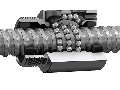
Power transmission screws—ball screws and lead screws—are typically used for converting rotary motion to linear motion. But when a load is applied axially to the nut, they do the opposite and convert linear motion to rotary motion. This is known as back driving. Depending on the application, backdrivability in ball screws could be an unwanted effect or a desired mode of operation. When using a ball screw as a mechanism to lift something we are probably interested on not having any backdrivability, however for some applications such as robotics mechanisms, grippers and so on, it could be interesting to have some backdrivability. For example on a gripper mechanism using a left-right ballscrew.
An axial force on the nut can cause a screw to back drive. Image credit: Thomson Industries
Ball screw and nut. Note circular thread profile and internal ball return. Source: SKF USA Inc.
What determines whether a screw will back drive?
Efficiency is the primary indicator of whether a screw will back drive or not—the higher the efficiency, the more likely the screw is to back drive when an axial force is applied. Two main factors play a part in determining a screw’s efficiency: the lead angle of the screw and the amount of friction in the screw assembly,
Lead angle—labeled “B” in the image below—is the angle between the helix of the screw thread and a line perpendicular to the axis of rotation.
Image credit: tools-n-gizmos.com
The chart below shows that the larger the lead angle, the higher the screw efficiency. In other words, screws with a higher lead (20 mm vs. 5 mm, for example) have a higher efficiency and, therefore, are more likely to back drive.
Lead angle vs forward efficiency for various friction coefficients. Image credit: THK
Friction in a screw assembly comes from seals, end support bearings, and drag torque from the nut itself. Although seals aren’t typically used on lead screws, lead screws do have higher drag torque than ball screws due to the fact that they rely on sliding (rather than rolling) contact. This means lead screws often have lower efficiencies, and as a result, are less likely to back drive than ball screw assemblies.
When does back driving matter?
In vertical applications, most drive mechanisms—such as belts, rack and pinion drives, and linear motors—will let the load “crash” or fall if power is lost to the motor. Screws, on the other hand, are less likely to allow the load to drop, and if they do (that is, if the screw is back driven by the load), it will occur at a somewhat controlled rate, since the friction in the assembly, the lead angle, and the inefficiency of the screw all must be overcome.
Determining if a screw will back drive is relatively simple: compare the back driving torque to the friction in the screw assembly. Back driving torque is based on the axial load, the screw lead, and the screw’s efficiency.
Where:
Tb = back driving torque (Nm)
F = axial load (N)
P = screw lead (m)
η2 = reverse efficiency*
*Efficiency when back driving is typically less than the efficiency for normal operation. Be sure to check the manufacturer’s specification for the back driving efficiency.
To determine the friction in the screw assembly, add the friction torque of the nut, seals, and end bearings—all of which can usually be found in the screw manufacturer’s catalog specifications. If the back driving torque is lower than the friction torque of the assembly, the screw is unlikely to back drive.
A rule of thumb for lead screws: if the lead is less than one-third the diameter of the screw, the screw is not likely to back drive.
A beginner roboticist should learn the basics of a few type of technologies and components before embarking himself in the design and construction of his own robot. I would say that the main areas one should be familiar with are:
Electric motors: it is important to distinguish the types and to know the basics of operation of the most used motors, e.g. DC brushed, DC brushless, PMSM, steppers, servos, etc. In a typical project, very frequently, one has to select the proper motor for an application and possibly the combination of motor and gearbox. I have published a very useful guide to select an electric motor for a simple robotic application. (https://enriquedelsol.com/2017/11/19/motor-selection-for-robots-i/).
Brushless motor
Motor controllers: the motors need to be powered and controlled with the right hardware, typically based on a H bridge made of transistors. It is important to understand the very basics of motor control to avoid spending a considerable amount of money in unnecessary hardware.
H bridge
Sensors: in robotics, it is a must to know the different sensors that can provide positional feedback, such as encoders, resolvers, potentiometers. Some of them will be needed depending on the motor we select for our application. In the simpler scenario of choosing servomotors, position sensors will only be needed as a backup sensing method. Other types of sensors very common are: temperature sensors, force sensors, velocity sensors (tachometers), linear displacement, light sensors, etc. It is very important to measure distance, in order to map the environment or to avoid obstacles. The most common sensors to measure distance are: infrared sensors (relatively inexpensive), ultrasonic sensors (inexpensive as well), lasers and depth cameras. These can measure the distance on a large interval to which they have been calibrated for. For an accurate distance detection, there are switches based on capacitive and inductive technology, very reliable but only available for fixed distances. Other common sensors that are used during the electronic control are current sensors and voltage meters.
This time I would like to review the most used online shops to buy components for a robotic design. Some of them are more focused on the professional market and some others pay attention to the hobbyist.
The two main companies that distribute components for the robotics industry and other engineering projects are RS (https://uk.rs-online.com/web/) and Farnell (https://www.farnell.com/). They are generalist companies oriented to the professional market with a very good client service, lead time and stock. Their search engines are very powerful and one can practically find everything they need. They are very well known in the European market and also established in the American market under other names: https://americas.rsdelivers.com/ , and https://www.newark.com/ . They usually offer free or very competitively priced next day delivery.
More focused on the hobbyist market, one can find RobotShop (https://www.robotshop.com) which has a deep and very well priced stock. It sells internationally. In this shop, the robotics enthusiast can find everything, from ready to assemble kits, to motors, sensors, cables, fixings, electronics, etc.
Another important reference in the hobbyist market is SparkFun (https://www.sparkfun.com/). Almost everything you may need can be found in this online shop, with special focus on electronic components.
If we need specialised hardware like wheels, structural elements, aluminium profiles, etc, a good online shop to buy from is Active Robots (https://www.active-robots.com/)
For an additional stock in electronics and mechanical components, I recommend to check Pololu (https://www.pololu.com), with a good range of components at a very competitive price.
Mouser (https://www.mouser.com/) and DigiKey (https://www.digikey.com/ ) are also two reference shops that work internationally, delivering plenty of products specially for the professional or the engineer. They are more focused in electronic components.
If we are looking for servos or ready to mount kits, we should check out Trossen Robotics, with a wide catalogue for the robotics enthusiast (https://www.trossenrobotics.com).
In addition to previous websites, the engineer or enthusiast should not forget the official distributor of Arduino (https://www.arduino.cc/) and the RaspberryPI official website (https://www.raspberrypi.org/), with tons of information about how to program their widely used development boards.
Depending on the desired component we are after, we can also review the website of the main manufacturers. For example, if there is plenty of budget available and we are looking for a motor, I would recommend checking out Maxon motors (https://www.maxongroup.com), with almost an infinite catalogue of electric motors of all types, electric drives and gearboxes. Other famous brands for the professional markets are Infranor (http://www.infranor.com/) and Yaskawa (https://www.yaskawa.com).
Hi, I would like to come back to my blog by commenting on very useful resources for the roboticist.
IEEE Spectrum: https://spectrum.ieee.org/ .The first one on the list. The IEEE is the world largest technical professional organization. They organise conferences, publish standards, and serve as a repository for an enormous amount of technical papers. Normally, when a researcher or just a curious person tries to access the papers in its brother website (ieee.org), they need to either pay a monthly/annual fee, or one-off payment to access the information. If the need is for professional use, your research centre or company should cover the expenses of the consultation or subscription. However, the IEEE Spectrum website can be enjoyed for free and it contains probably the best summary of new discoveries, advances and new trends in robotics and related industries. It is however, biased towards the American research.
Robohub: https://robohub.org/ .Robohub is a non-profit organisation that as its name says, it is a hub for sharing stories, news, research, articles and interviews about robotics. It brings together experts in robotics to make sure the contents meet the highest editorial standards. They claim that their information is original and does not appear anywhere else. It is a good source of educational resources. It also has a very good podcast at: https://robohub.org/podcast-episodes/.
org: The Robotic Industries Association posts daily news, case studies, technical papers, job openings and much more. It has a very good section about news in emerging markets and industry standards ( https://www.robotics.org/).
Robotics Business Review: The Robotics Business Review claims to be “The Largest, Most Comprehensive Online Robotics News and Information Resource“. It regularly posts about all aspects of the business of robotics. However, most of its posts are only short abstracts and you must pay a yearly membership fee to access the complete article ( https://www.roboticsbusinessreview.com/).
The Robot Report: The Robot Report is written by roboticist, Frank Tobe, cofounder of Robo-Stox, a tracking index for the robotics industry, now RoboGlobal. Through the blog he aims to follow the business of robotics and regularly reports on developments from all areas of the robotics industry.( https://www.therobotreport.com/)
Machine Design: (machinedesign.com/). The technical quality of this blog / website is impressive. They provide a general knowledge of different fields in robotics, automation and engineering. It is a good source of technical articles and also news about the industry. If anyone is looking to explore more in-depth the technical issues behind robotics this is the place to go.
For the people interested in attending to conferences, workshops or looking for jobs in the robotics industry, there are two mail lists where every event is published. These are:⅞
Encoders, whether rotary or linear, absolute or incremental, typically use one of two measuring principles—optical or magnetic. While optical encoders were, in the past, the primary choice for high resolution applications, improvements in magnetic encoder technology now allow them to achieve resolutions down to one micron, competing with optical technology in many applications.Magnetic technology is also, in many ways, more robust than optical technology, making magnetic encoders a popular choice in industrial environments.
Parameter
Optical Sensor Characteristics
Magnetic Hall Sensor Characteristics
Principle
coded disc/scale, through beam arrangement
magnet/tape/polewheel opposed to sensor
Incremental accuracy of target
100 nm – 1 μm
(lithography process)
5 μm – 30 μm
(magnetisation process)
Energising
by external LED (20 mW)
by target (Br>220 mT)
Signal Frequency
> 1 MHz possible
< 50 kHz
Benefits
high code density, high code accuracy
robust
Disadvantages
sensitive to contamination, high alignment requirements
Electrical noise is a common problem that occurs during the transmission of an incremental encoder’s signal to the receiving electronics, especially when the cable lengths are very long. Stray electromagnetic fields or currents induce unwanted voltages into the signal. These voltages can cause the receiver to make false counts, producing errors in the position or velocity feedback.
The primary way to alleviate electrical encoder noise is to use TTL output – also known as differential line driver output. This output format provides not only the standard A and B square wave signals and a Z reference signal, it also includes their complementary signals, /A, /B, /Z (sometimes written as A’, B’, and Z’). These complementary signals are produced by splitting the output of each channel (A, B, and Z) into two signals that are 180 degrees out of phase (complements) with each other. In other words, when the A signal is high (logic state 1) the A’ signal will be low (logic state 0). The receiving electronics take the state of that channel as the difference between the two signals.
In order for the complementary signals to be read, however, the receiving electronics must have a circuit that is designed for differential input – known as line receiver input. In addition, the wires for each channel (A and A’, for example) should be a twisted pair. In this twisted pair of wires, any electrical encoder noise that is induced will be the same on each signal. The receiving electronics recognise only the difference between the two signals, and because the signals are complements (equal in magnitude, with 180 degree phase lag) but the noise is common mode (equal on each signal, with no phase lag), the noise is cancelled out on the receiving end.
Incremental quadrature encoder for noise rejection
The trend towards wide scale use of Brushless Motors is being driven by manufacturing
cost reductions, improved efficiencies, greater reliability, availability of improved drive
electronics, and the availability of improved sensors for motor control.
The brushless motors, independently whether they are PMSM or BLDC motors, require to know the relative position of the windings with respect the motor poles. To do this, a set of Hall Effect sensors are typically employed and placed between windings. An alternative option is to use the positional feedback from more accurate sensors to determine the presence of the magnetic field without using Hall Effect sensors. However, an intelligent drive is required to perform this count and issue the signal that conmutates the phases. This action is performed automatically with the bipolar Hall-Effect sensors.
Hall Effect sensor
For the majority of applications in the US and Japan, the trend in brushless motor sensor designs is moving away from Hall boards and feedback elements to integrated devices. For resolver applications, it can be handled by adding a dedicated set of 2, 3, or 4 speed windings for commutation, or it can be handled with a single speed winding and an intelligent drive.
The elimination of the Hall sensors from the BLDC motor eliminates many of the potential problems which can occur in a motor application. Hall devices are sensitive to acoustic noise, current spikes, temperature, EM fields, and can be difficult to align, which results in torque ripple. When a BLDC motor is used in a servo application with a high resolution feedback sensor, Hall sensors are redundant and consume space. They also add to motor length, assembly costs, cable harnessing complexity, and decrease overall reliability. The use of an encoder or resolver to eliminate Hall sensors in this situation is not only cost effective, but also improves the overall system performance.
Drive with Hall board, Encoder or Resolver for Commutation and Feedback a caption
Drive with Commutating Encoder
Encoder Types.
When an encoder is used as the feedback element, there are a variety of types to choose from. The following is a short summary of the predominant types currently available.
1. Incremental, (TTL)
Readily available from a wide variety of Suppliers. Almost unlimited line count availability up to 5000 cycles per revolution. Special line counts and output options
are easily obtained.
2. Incremental with Commutation, (TTL)
Becoming more common in the US and Japan, availability is somewhat constrained by lack of industry standards. Mounting configuration, signal conditioning, and power supplies vary widely. Available in line counts up to 8000 for 2, 4, 6, and 8 pole motors. They are being developed in both hollow-shaft and modular versions by a variety of encoder suppliers.
3. Incremental with Commutation, (Sine wave)
More common in Europe, this type of encoder generally has sinusoidal quadrature
outputs, with a 1 volt pk-pk amplitude. Commutation is accomplished using a quadrature one cycle per revolution output.
4. Absolute Single Turn, (TTL/Parallel)
Less common for drive applications, these are usually found in 10 to 12 bit versions. Larger word sizes are available, but costs become a real issue and make them unsuitable for all but the most specialized applications.
5. Absolute Multi-turn, (Sine wave Incremental, Serial Absolute)
These encoders are generally based upon a 12 or 13 bit single turn absolute encoder, with a 12 bit turn counter yielding 24 or 25 bits of position information. Although these have been available for some time, they have been too costly for widespread applications. Recent developments in Europe, however, are making these more available, and costs are starting to come down. These encoders contain an incremental output with A, B, and Reference pulse, a serial absolute interface, and commutation outputs. Commutation output is derived from the MSB of the single-turn absolute. The Incremental tracks are derived from the LSB of the absolute encoder, and generally result in a 2048 or 4096 cycles per revolution incremental signal that is suitable for use in high-speed servo controls.
One of my mates is developing several projects related to robotics which are worth mentioning. In his blog, one of his last projects is the construction of an humanoid robot based on steppers.
Upgraded X-carriage and extruder V1 (Complete layout)
Figure 7. Improved X-Carriage
Dexter Manipulator manufactured by Oxford Technologies Ltd.
Olympus videoscope.
HoneyBee pipe inspection robot
ABB robot with a closed loop.
Robotics & Mechatronics explanatory diagram including the involved areas such as: mechanical design, electronics, control systems and artificial intelligence.
HoneyBee pipe inspection robot
Kraft GRIPS hydraulic manipulator with force feedback