The simplest velocity estimation method is the Euler approximation that takes the difference of two sampling positions divided by the sampling period. Typically the position measurements are taken with encoders or resolvers which contain stochastic errors which result in enormous noise during the velocity estimation by the Euler approximation when the sampling period is small and the velocity low [1] .

Encoder
Different alternatives have been tried which utilise more backwards steps to reduce the noise but introducing a small delay. On [3] a first order adaptive method is shown which is able to vary the backward steps depending on the speed. Also, on [2] it has been found that 3 steps is the best for a sampling rate of 2500 Hz in their experiments with an encoder of 655360 pulses per revolution. They also implemented a Kalman observer and non-linear observers, obtaining the same results than an averaging of the Euler formula. On [4] a Kalman filter is tested assuming a normal distribution of the position error. On [1] a dynamic method which varies the samples used for averaging depending on the speed is developed with very good results. For example, given a desired relative accuracy 

time kT is given by θ(k). The relative accuracy is given by:
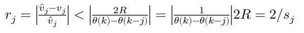
Where 

[1] G. Liu. “On velocity estimation using position measurements”. In: Proceedings
of the american control conference, Anchorage, AK May 8-10. 2002, vol. 2, pp. 1115-
1120.
[2] A. Jaritz, M.W. Spong. “An experimental comparison of robust control algorithms on a direct drive manipulator”. In: IEEE Transactions on Control Systems
Technology. 1996, vol.4, no.6, pp.627-640. doi: 10.1109/87.541692
[3] F. Janabi-Sharifi, V. Hayward, C-S.J. Chen. “Discrete-time adaptive windowing for velocity estimation”. In: IEEE Transactions on Control Systems Technology.2000, vol.8, no.6, pp.1003-1009. doi: 10.1109/87.880606
[4] P.R. Belanger, P.Dobrovolny, A. Helmy, and X. Zhang. “Estimation of angular
velocity and acceleration from shaft-encoder measurements.” The International Journal
of Robotics Research. 1998, vol. 17, no. 11, pp. 1225-1233


Leave a comment